Re-Scoring an ML Detection Engine on Past Attacks, Part 2

This is the second of two posts on ML Re-scoring at Abnormal. If you haven’t read Part 1 yet, you may want to check it out before continuing.

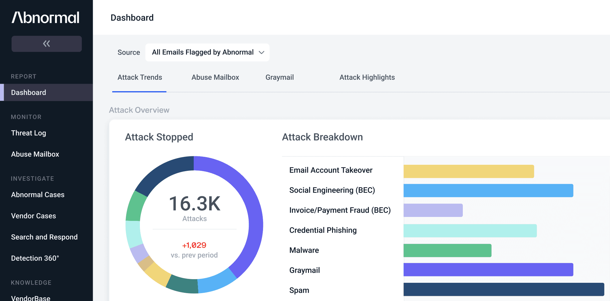
In Part 1 of this blog post, we set the stage for the complex cybersecurity problem we’re solving, and why our ML solution requires an efficient and unbiased re-scoring pipeline. To recap, our ML pipeline powers a detection engine that catches the most advanced email attacks. These attacks are not only extremely rare, but also change over time in an adversarial way. Since we require both high precision and high recall, and the cost of any error is severe, it is essential to have a system that can continuously re-evaluate our ML system to ensure that it’s always up to our standards. This kind of re-scoring system is also an essential part of the MLOps process that greatly improves the speed with which an ML engineer can take a prototyped feature to production.

In the first post, we also established that this is a big data problem with some tricky requirements. The system should:

1. Update all historical messages with the latest attribute extraction code, joined datasets, and model predictions,
2. Perform all of these computations just as our current online system would,
3. With time travel, i.e. evaluate all messages as they would have looked at original scoring time, and
4. Do all of this efficiently enough to enable rapid development.

In this second post, I’ll take a deep dive into why implementing a re-scoring system that meets these requirements is such a challenge and how we’ve solved it at Abnormal. I’ll also show that this can all be done without any special-purpose systems, using only the standard set of tools provided by Spark. Still, this won’t be an easy task, and we’ll see that it’s necessary for data engineers to invest greatly to make this re-scoring system a platform that’s as easy for ML engineers to use as traditional CI/CD.

Gathering Historical Advanced Email Attacks

Let’s start with the first requirement—we need to process every labeled message we’ve ever seen so that each one can be run through an offline simulation of our scoring pipeline. The source of truth for historical messages is a real-time database that gets updated with attack messages and their labels as we detect them. For a few reasons, our first step will have to be copying these messages and labels into a more flexible environment. In particular:

1. We’ll need to run Python code on these historical messages in order to re-extract features and re-run our models,
2. There are more than enough messages to make doing so very slow on a single machine, and
3. We require other datasets that aren’t in this database, and aren’t suitable for it anyway.

At Abnormal, our distributed data processing platform of choice is Apache Spark, which lets us run custom code in parallel across many machines, pulling in any data that is required. This solves all three problems mentioned above, so we’ll start our ETL pipeline by copying our messages and labels into an environment where we can run Spark. In this case, we run an Apache Sqoop job to copy messages and labels from the database into our data lake, from which Spark can quickly read in distributed files in parallel. As an aside, in reality, we’ll have a snapshot of a table with messages, and another of labels. In order to join in labels with some custom Python logic, we actually join messages with labels in Spark too.

From this point on, we’ll be able to run any Python code we want over our historical labeled messages, pull in any external data sources, and do all of this in an efficient, parallel way. Now, the work remaining is to simulate our online scoring pipeline accurately and without bias. At a high level, the steps required to do this are to

1. Join in all the data that’s available online, with time travel, and
2. Re-run all the attribute extraction and model scoring code.

A simplified view of the whole pipeline would look like this:

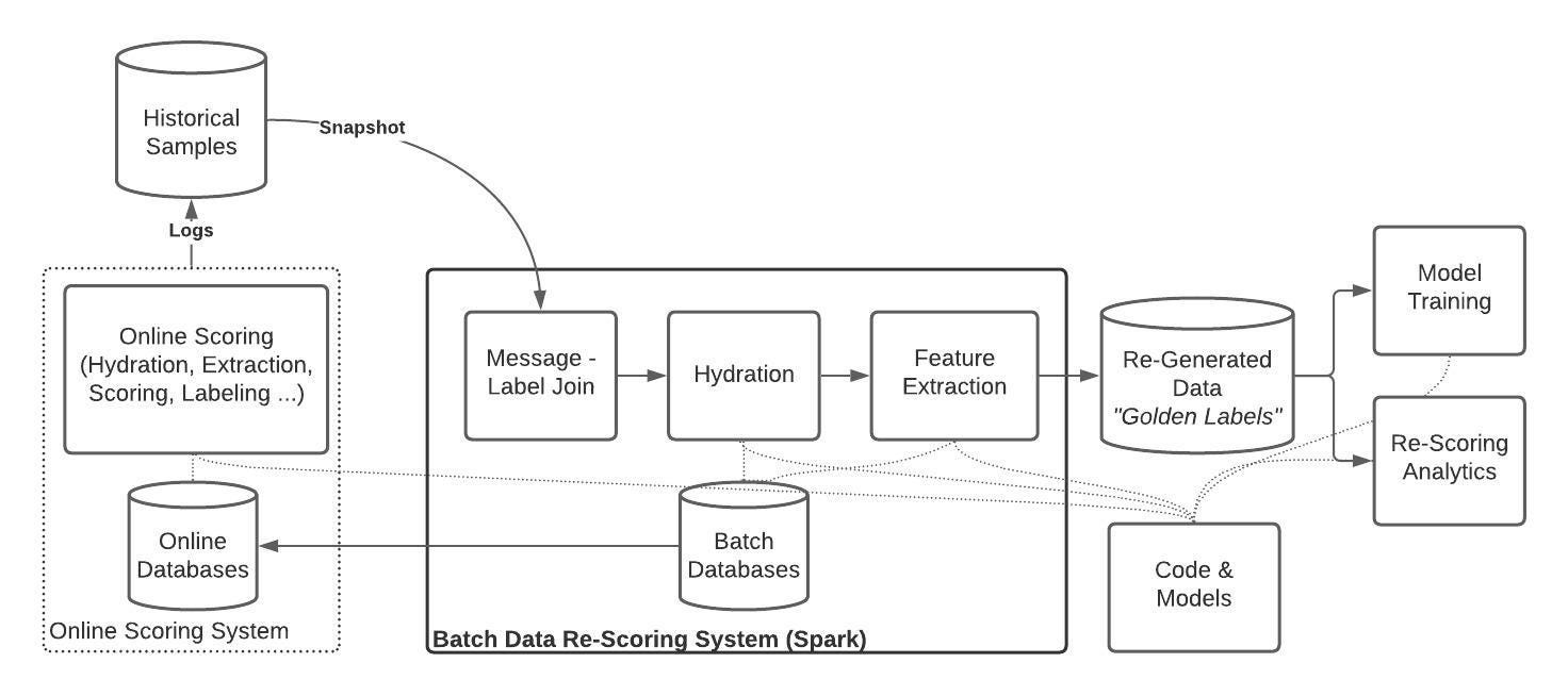
From an implementation perspective, the most challenging of these stages turns out to be accurately joining in all the datasets our models require. However, with some careful logic, we’ll show how this can be done only using Spark.

Re-hydrating Advanced Email Messages

In order to make our online predictions as effective as possible, we join in quite a bit of data to provide further context about the email that’s being evaluated. The raw email will have some basic attributes like the sender’s display name and email address, but there’s lots of further context that can make it clear when something abnormal might be happening.

For example, an ML engineer might come up with a feature that counts the number of times an email has been seen in the last 30 days; if an email is from an address that has never been seen before, our models may learn that it’s more suspicious. Let’s call this feature 30d_EMAIL_COUNT. The ML engineer might build a test dataset of email counts, prototype a new model feature, and train a model with it. But now, how can the engineer get the new feature into production?

In our online system, we use a variety of in-memory and remote data stores to serve data for hydration and there’s a great set of tooling to make it easy to start serving new features. But how can the ML engineer do the same in our re-scoring system? This is an essential part of the MLOps process—the ML engineer needs to know how the new feature affects our detection engine’s performance on historical messages—but joining in this new dataset is a hard problem for two reasons:

1. The Big Data Join Problem: Generally, these databases are large key-value stores that are used online as row-based lookups. When re-hydrating large sets of samples in batch, we need to do a large join.
2. The Time Travel Problem: For aggregate features, it’s not enough to join the most recent value of that aggregate to our samples. Take for example the 30d_EMAIL_COUNT attribute we discussed above, and consider two emails A and B. Both of these emails A and B are from “xyz@gmail.com”, but A was received today, and B was received 1 week ago. To hydrate email A with 30d_EMAIL_COUNT we want to look up the count of emails from this address in the past 30 days. For email B, we would like to look up the count starting from 1 week ago and going 30 days back from there. Clearly, if we are to use today’s count of the latter message it will be incorrect—most obviously, today’s count will include the email in question. This is the time travel problem. How do we rewind our databases to the correct point in time to create the right features?

We’ll show how these problems can be solved using just Spark, but we’ll also come to the conclusion that the ML engineer should never have to think about doing so.

Joining Offline Datasets

Spark provides a set of functionality that allows us to solve the big data join problem. For “small data” we use either of Spark’s options for copying data to each machine—broadcast variables for in-memory data, and SparkFiles for on-disk data.

A broadcast variable sends a given variable to every executor for use in-memory:

# Broadcast variable to every executorsmall_ip_dataset = {“1.2.3.4”: 123, “5.6.7.8”: 567}ip_broadcast = sc.broadcast(dataset1)# hydrate_with_ip_count can use the small_ip_dataset dictionaryhydrated_rdd = rdd.map(lambda message: hydrate_with_ip_count(message, ip_broadcast.value))

While a SparkFile asks every executor to download a file to disk:

from pyspark import SparkFiles# Add Spark file so that every executor will download itsc.addFile(remote_dataset_path)# Now the file can be loaded in any Spark operation from local_dataset_pathlocal_dataset_path = SparkFiles.get(os.path.basename(remote_dataset_path)[: -len(".tar.gz")])

SparkFiles are most useful when the data is in a format that’s easiest to work with from disk, like a RocksDB.

These two cases are easy enough for any ML engineer to get working quickly enough. But when the size of the datasets is larger than about 100 MB, we consider it a “big data join” and use a proper Spark join operation, and things start to get complicated quickly.

Solving the Time Travel Problem

For a subset of our datasets, the risk of online and offline logic diverging becomes even greater because data may change over time. As we described above in the 30d_EMAIL_COUNT example, messages should be re-hydrated exactly as they would have been during online scoring.

To solve this time travel problem, it’s necessary to time index data with an acceptable level of granularity and perform a join as-of event time. For the 30d_EMAIL_COUNT data, let’s say we’re okay with daily granularity. This means that a message appearing on day t should be joined with the sum of counts over days [t-30, t). To perform this join, then, the first step is to pre-compute this sliding 30-day sum for each day:

Here, the y-axis represents the value of each count, and the x-axis represents time. Different colors denote different feature values; in the 30d_EMAIL_COUNT example, these would be different email addresses.

Next, since every event must be joined by event time and its particular feature value (again, email address in our example), we’ll key our events by day and by email address:

And at this stage, we now have two datasets with matching join keys, a tuple of time, and feature value. Now it’s just necessary to perform the join. A sketch of our time-travel join logic in Spark looks something like this:

# Index every event by key and day, and take event ID to avoid passing around large objectskeyed_event_id_rdd = _expand_events_by_key_day(event_rdd)# Index every count by key and daykeyed_counts_rdd = _expand_counts_by_key_day(time_sliced_counts_rdds)# Join date-indexed event ID’s with date-indexed counts, by common keyjoined_event_id_and_daily_counts_rdd = keyed_event_id_rdd.leftOuterJoin(keyed_counts_rdd)# In memory, sum up cumulative counts and key by event IDcumulative_counts_by_event_id_rdd = joined_event_id_and_daily_counts_rdd.flatMap(_extract_cumulative_counts)# Join actual events back in by event IDjoined_event_and_cumulative_counts_rdd = cumulative_counts_by_event_id_rdd.join(event_rdd.keyBy(_get_id_from_event))# Hydrate every event with cumulative countshydrated_events_rdd = joined_event_and_cumulative_counts_rdd.map(_hydrate_event_with_counts)

As promised, using basic Spark operations, we’re able to re-hydrate messages with all the data our models require, and to do so in an unbiased way.

A Playbook for Joining Data

While we were able to do all of this in Spark, it’s useful to go through this exercise because it shows just how complicated this process can get. You may even notice that the sketch of the Spark code above is even more convoluted than the sketch we described in the preceding diagrams. It turned out that that naive approach didn’t scale well, and so even more logic to first join by event ID rather than full event was required.

In any case, we would never expect a software engineer to go through all this trouble just to add a unit test for their code. Adding re-scoring coverage for a new feature is just as important as adding test coverage for a new code, and it has to be just as easy.

The job, then, for a data engineer building a re-scoring system is to make the process of adding new data to the re-scoring system dead-simple. At a high level, data engineers can offer a playbook that looks something like this:

The “small data” joins are just a couple lines of code, and simple enough for an ML engineer to add to the re-scoring system in a reasonable amount of time. But, as we showed, implementing a full Spark join with time travel is a complex process. An essential part of the re-scoring system is a set of plug-and-play Spark code that any ML engineer can use to incorporate even a huge dataset without having to think about a dozen join and map operations.

In fact, we should be able to standardize the Spark code showed above and provide an interface that only requires a few functions particular to the data at hand:

class TimeSlicedStatsEventHydrater(Generic[Stat, Event]): # How to build the keys to join on _lookup_stats_builder: LookupStatsBuilder
 # How to hydrate the Event with the Stats _hydrate_event: EventHydrater
 # How to extract the date from an event _get_date_from_event: DateExtractor
 # How to extract the ID from an event _get_id_from_event: IdExtractor

This is now a much more reasonable amount of work to be done by an ML engineer testing a new feature.

Re-running Attribute Extraction and Model Scoring

After the re-hydration stage, our work is mostly cut out for us, at least from a data engineering perspective. We still need to re-extract attributes for our messages based on the latest code, and then re-run our prediction stack using the latest models. This process of extraction and scoring is extremely sophisticated under the hood, but from the perspective of a Spark job, it’s as simple as mapping a function over every message. In reality, there are some engineering challenges involved in setting up our scoring system in Spark, but they’re outside the scope of this post.

After applying this function, we finally have a fully re-scored dataset of historical messages. Every re-processed message has its original, canonical label, plus freshly re-joined data and re-extracted attributes, and a new judgment that reflects our latest scoring system. As discussed in the previous post, this dataset is invaluable, as it allows our data scientists and engineers to continuously monitor detection performance and train future ML models. Both of these downstream use-cases bring their own interesting challenges, but for now, we’ll leave these topics for later blog posts.

Finally, if you’re interested in the machine learning, data engineering, and many other challenges we’re solving at Abnormal, we’re hiring!

Thanks to Jeshua Bratman, Carlos Gasperi, Kevin Lau, Dmitry Chechik, Micah Zirn, and everyone else on the detection team at Abnormal who contributed to this pipeline.